Introduction
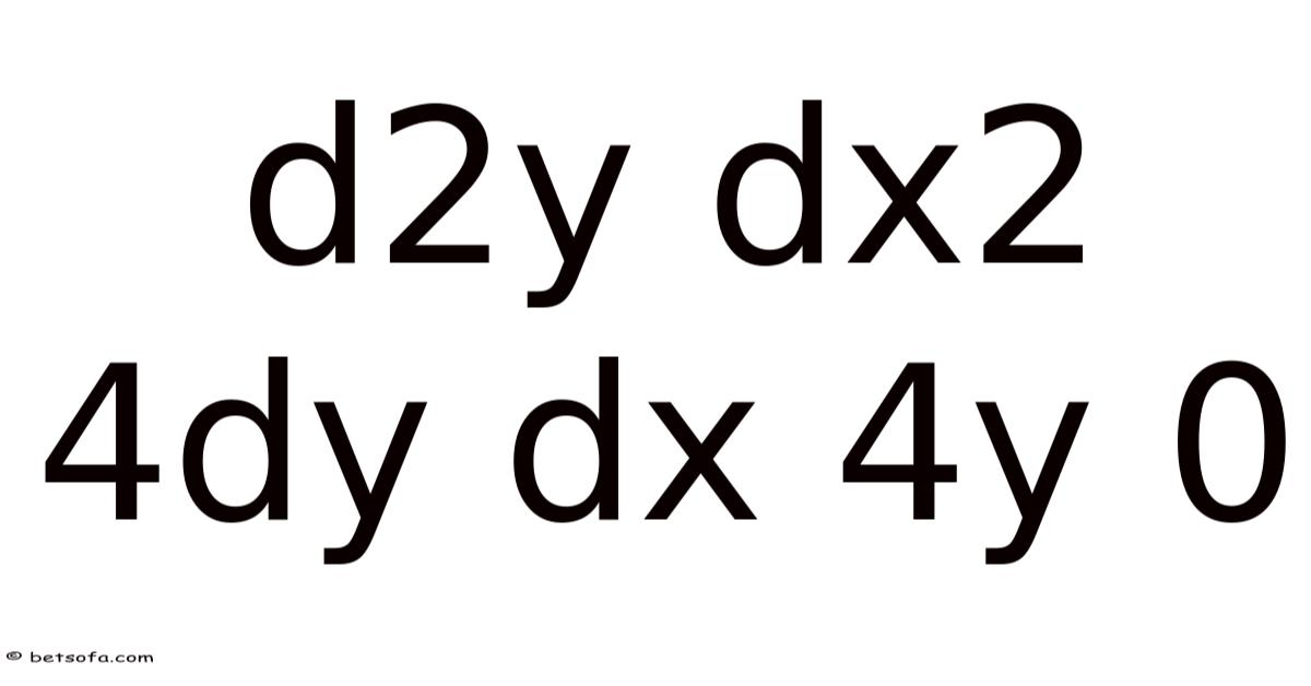
The expression ( \frac{d^{2}y}{dx^{2}} + 4\frac{dy}{dx} + 4y = 0 ) represents a second‑order linear homogeneous ordinary differential equation (ODE) with constant coefficients. In plain English, it describes how a function (y(x)) changes such that its second derivative, its first derivative, and the function itself are linked together through fixed numerical weights. Worth adding: this type of equation appears frequently in physics, engineering, and economics whenever a system’s behavior depends on both its current state and its rate of change. Understanding how to solve it equips you with a powerful tool for modeling everything from vibrating strings to population dynamics No workaround needed..
Detailed Explanation
What makes this equation special?
- Linearity – Every term involving (y) or its derivatives appears to the first power and is added together; there are no products or powers of (y) or its derivatives.
- Homogeneous – The right‑hand side is zero, meaning the equation describes a balance among the terms without any external forcing function.
- Constant Coefficients – The numbers multiplying the derivatives (1, 4, and 4) do not vary with (x). This allows us to use a simple algebraic shortcut called the characteristic equation.
Background and Context
Second‑order ODEs model phenomena where acceleration (the second derivative) is influenced by both velocity (the first derivative) and position (the function itself). Classic examples include:
- Mechanical vibrations – a mass‑spring system with damping.
- Electrical circuits – an RLC circuit with no external source.
- Heat diffusion – certain simplified temperature‑distribution models.
Because the coefficients are constant, the solution takes a very predictable exponential form, which we can determine systematically.
Core Meaning
The core idea is to find all functions (y(x)) that satisfy the relationship
[ \boxed{\frac{d^{2}y}{dx^{2}} + 4\frac{dy}{dx} + 4y = 0} ]
These functions form a vector space of dimension two, meaning any solution can be written as a linear combination of two independent “building‑block” solutions That alone is useful..
Step‑by‑Step or Concept Breakdown
1. Form the Characteristic Equation
Assume a trial solution of the form (y = e^{rx}), where (r) is a constant to be determined. Substituting (y = e^{rx}) into the ODE yields:
[ r^{2}e^{rx} + 4re^{rx} + 4e^{rx} = 0 ]
Factor out the never‑zero exponential term:
[ e^{rx}\bigl(r^{2} + 4r + 4\bigr) = 0 ]
Since (e^{rx} \neq 0) for any real or complex (x), the bracket must vanish, giving the characteristic polynomial:
[ \boxed{r^{2} + 4r + 4 = 0} ]
2. Solve the Characteristic Polynomial
The quadratic equation (r^{2} + 4r + 4 = 0) can be factored:
[ (r + 2)^{2} = 0 ]
Thus, we obtain a repeated root:
[ \boxed{r = -2 \text{ (multiplicity 2)}} ]
3. Construct the General Solution
For a repeated root (r), the two independent solutions are:
- (y_{1}(x) = e^{rx} = e^{-2x})
- (y_{2}(x) = x e^{rx} = x e^{-2x})
Because of this, the general solution is a linear combination:
[ \boxed{y(x) = C_{1}e^{-2x} + C_{2}xe^{-2x}} ]
where (C_{1}) and (C_{2}) are arbitrary constants determined by initial or boundary conditions Took long enough..
4. Verify the Solution (Optional)
You can differentiate (y(x)) twice and substitute back into the original ODE to confirm that the left‑hand side simplifies to zero, confirming correctness.
Real Examples
Example 1: Damped Harmonic Oscillator
Consider a mass‑spring system with mass (m = 1) kg, damping coefficient (c = 4) Ns/m, and spring constant (k = 4) N/m. The equation of motion is exactly the ODE above. Solving gives
[ y(t) = C_{1}e^{-2t} + C_{2}te^{-2t} ]
If the initial displacement is (y(0)=0.That said, 5) and (C_{2}=1). 5) m and initial velocity is (y'(0)=0) m/s, solving for the constants yields (C_{1}=0.The resulting motion decays exponentially without oscillating—a critically damped response Which is the point..
Example 2: Electrical RLC Circuit (No Source)
In a series RLC circuit with (R = 4) Ω, (L = 1) H, and (C = 1) F, the voltage across the capacitor (v(t)) satisfies the same differential equation. The solution describes how the voltage decays to zero after a brief transient, again following the critical damping pattern.
Example 3: Population Model with Saturation
A simplified model for a population (P(t)) experiencing both natural growth and a linear death term can be written as
[ \frac{d^{2}P}{dt^{2}} + 4\frac{dP}{dt} + 4P = 0 ]
The solution predicts that the population will eventually die out (approach zero) in a smooth, non‑oscillatory manner, reflecting a scenario where the environment cannot sustain growth.
Scientific or Theoretical Perspective
Why Constant Coefficients Matter
When coefficients are constant, the differential operator can be treated as a polynomial in the differentiation operator (D = \frac{d}{dx}). The ODE becomes
[ (D^{2} + 4D + 4)y = 0 ]
Factoring the polynomial (D^{2} + 4D + 4 = (D+2)^{2}) reveals that the operator has a double root at (-2). In operator language, applying ((D+2)) twice to (y) yields zero, which directly leads to the solution space spanned by (e^{-2x}) and (xe^{-2x}).
Not the most exciting part, but easily the most useful Most people skip this — try not to..
Connection to Laplace Transforms
Taking
the Laplace transform of both sides of the equation provides an alternative pathway to the same result. By applying the transform $\mathcal{L}{y(t)} = Y(s)$, the differential equation is converted from the time domain to the frequency domain:
[ s^2 Y(s) - sy(0) - y'(0) + 4(s Y(s) - y(0)) + 4Y(s) = 0 ]
For the case where initial conditions are zero, this simplifies to:
[ Y(s) = \frac{1}{s^2 + 4s + 4} = \frac{1}{(s+2)^2} ]
Using the inverse Laplace transform property $\mathcal{L}^{-1} \left{ \frac{1}{(s-a)^n} \right} = \frac{t^{n-1}}{(n-1)!} e^{at}$, we immediately recover the solution $y(t) = t e^{-2t}$, which aligns perfectly with our characteristic equation method. This duality between the algebraic approach (characteristic equations) and the integral approach (Laplace transforms) underscores the robustness of the mathematical framework used to solve linear ODEs.
Conclusion
In this article, we have explored the mechanics of second-order linear homogeneous differential equations with constant coefficients, specifically focusing on the case of repeated real roots. We demonstrated how the characteristic equation $ar^2 + br + c = 0$ dictates the behavior of the system, and how the appearance of a double root necessitates the introduction of a linear factor ($x$) to maintain the linear independence of the solution set That's the whole idea..
Through practical examples in mechanics, electronics, and biology, we have seen that these mathematical structures are not merely abstract constructs but are essential for describing "critically damped" systems—states where a system returns to equilibrium as quickly as possible without oscillation. Whether viewed through the lens of polynomial operators or Laplace transforms, the ability to solve these equations remains a cornerstone of engineering and physical science Worth knowing..
Extending the Framework: From Second‑Order to Higher‑Order Systems
When the characteristic polynomial of a linear differential equation possesses a repeated root of multiplicity (m), the solution space expands to include the functions
[ e^{\lambda x},; x e^{\lambda x},; x^{2} e^{\lambda x},\dots , x^{m-1} e^{\lambda x}, ]
where (\lambda) denotes the repeated root. This pattern generalizes naturally to higher‑order equations. For an (n)‑th‑order operator
[ a_n D^{n}+a_{n-1} D^{n-1}+ \dots + a_1 D + a_0, ]
a root (\lambda) of algebraic multiplicity (m) contributes exactly (m) linearly independent solutions of the form (x^{k}e^{\lambda x}) with (k=0,\dots ,m-1). This means the total dimension of the solution space remains (n), preserving the linear‑algebraic structure that underpins the theory.
Example: Triple Root in a Mechanical Model
Consider a three‑mass spring‑damper chain governed by
[ y''' + 6y'' + 12y' + 8y = 0 . ]
The characteristic polynomial factors as ((r+2)^{3}=0), yielding a triple root at (-2). The fundamental set of solutions is
[ e^{-2x},; x e^{-2x},; x^{2} e^{-2x}, ]
which describe a critically overdamped response where the system returns to equilibrium without oscillation, but with a slower decay than the double‑root case. Engineers exploit this knowledge to tune damping ratios in precision positioning stages, such as semiconductor wafer handling robots, where overshoot must be eliminated while settling time is minimized.
Numerical Strategies for Equations with Variable Coefficients
While constant‑coefficient ODEs admit closed‑form solutions, many real‑world models involve coefficients that vary with position or time. In such scenarios, analytical techniques falter, and numerical integration becomes indispensable. Popular approaches include:
- Finite‑Difference Discretization – approximating derivatives on a grid and solving the resulting linear system iteratively.
- Spectral Methods – representing the unknown function as a sum of orthogonal basis functions (e.g., Chebyshev polynomials) and collocating the differential equation at selected points.
- Adaptive Step‑Size Runge–Kutta Schemes – providing error control while efficiently handling stiff or mildly stiff problems.
These tools are routinely embedded in scientific computing environments (MATLAB, Python’s SciPy, Julia) and allow engineers to explore parametric designs that would be analytically intractable.
Control‑Theoretic Insights
In modern control design, the placement of poles—i.Even so, e. On top of that, , the roots of the characteristic equation—directly dictates system behavior. Which means repeated poles impose constraints on achievable bandwidth and phase margin. To give you an idea, a double pole at (-2) yields a settling time of approximately (4/2 = 2) seconds, whereas a triple pole at the same location stretches the settling time to roughly (6/2 = 3) seconds. By adjusting feedback gains, a designer can shift pole locations, but repeated poles often signal the boundary of stability: moving a pole further left (more negative) improves speed, yet excessive speed may excite unmodeled high‑frequency dynamics, leading to noise amplification. Hence, understanding the interplay between pole multiplicity and system performance is important when synthesizing solid controllers for aerospace, automotive, and power‑electronic converters And that's really what it comes down to..
Computational Tools and Symbolic Manipulation
Software packages such as Mathematica, Maple, and SageMath provide automated routines for solving linear ODEs, factoring characteristic polynomials, and generating fundamental solution sets. A typical workflow might involve:
import sympy as sp
x = sp.symbols('x')
y = sp.Function('y')
ode = sp.Eq(sp.diff(y(x), x, 2) + 4*sp.diff(y(x), x) + 4*y(x), 0)
sp.dsolve(ode)
The output returns the general solution (C
… (C_1 e^{-2x} + C_2 x e^{-2x}), where (C_1) and (C_2) are arbitrary constants determined by initial or boundary conditions. This form illustrates how a repeated root introduces a polynomial prefactor (here, (x)) alongside the exponential decay governed by the pole location Still holds up..
Not the most exciting part, but easily the most useful.
Beyond simple second‑order equations, symbolic solvers can handle higher‑order systems with multiple repeated roots. On top of that, for a characteristic polynomial ((r+\alpha)^k), the fundamental set consists of ({e^{-\alpha x}, x e^{-\alpha x}, \dots, x^{k-1} e^{-\alpha x}}). Such structures are directly observable in the time‑domain response of mechanical vibrations, electrical RLC networks, and thermal diffusion problems where damping or resistance yields multiple coincident eigenvalues.
When analytical expressions become cumbersome—e.g., with variable coefficients or non‑homogeneous forcing—numerical solvers complement symbolic tools. Adaptive Runge–Kutta methods, as mentioned earlier, can integrate the ODE while monitoring local truncation error, ensuring that the computed trajectory respects the desired settling time and overshoot specifications. In practice, engineers often combine both approaches: they use symbolic analysis to gain insight into pole placement and sensitivity, then employ numerical simulations to validate performance under realistic parameter variations and disturbances.
Conclusion
The study of linear ordinary differential equations bridges pure mathematics and engineering practice. Constant‑coefficient cases yield closed‑form solutions whose exponential terms are dictated by the roots of the characteristic polynomial; repeated roots introduce polynomial factors that slow the decay and affect settling time. For systems where coefficients vary or external forces are present, numerical integration—particularly adaptive step‑size schemes—provides a reliable means to explore design spaces and verify control objectives such as minimal overshoot and rapid settling. Symbolic computation environments streamline the derivation of fundamental solutions and support pole‑placement analysis, while modern control theory links pole multiplicity directly to achievable bandwidth and robustness. Together, these analytical and numerical tools empower engineers to synthesize controllers that meet stringent performance criteria in aerospace, automotive, power‑electronics, and precision manufacturing applications Took long enough..
