Introduction
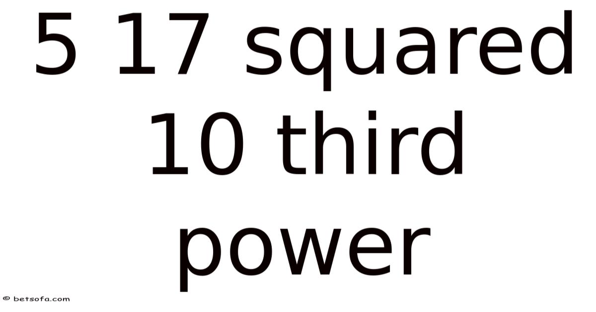
Understanding 5 × 17² × 10³ is more than just a quick arithmetic exercise; it illustrates how powers, multiplication, and scaling interact in both everyday calculations and scientific contexts. This expression combines three distinct operations: squaring a whole number, raising another number to the third power, and then multiplying the results together with a leading coefficient. By dissecting each component, you’ll see how the final value of 1,445,000 emerges naturally, and you’ll gain a reusable framework for tackling similar problems in finance, physics, engineering, and data analysis.
Detailed Explanation
The notation 5 × 17² × 10³ can be read as “five times seventeen squared times ten cubed.”
- 17² means “seventeen squared,” i.Even so, e. Which means , 17 multiplied by itself. - 10³ means “ten raised to the third power,” i.e.Consider this: , ten multiplied by itself three times (10 × 10 × 10). - The leading 5 acts as a multiplier that scales the product of the two powers.
When you evaluate the expression step‑by‑step, you first compute the powers, then multiply the results. Here's the thing — the background of such expressions lies in algebraic notation, where coefficients, bases, and exponents are combined to represent repeated multiplication compactly. But this order follows the standard hierarchy of operations (exponents before multiplication). In scientific notation, powers of ten are especially important because they shift decimal points, making large or tiny numbers easier to read and manipulate.
Step‑by‑Step or Concept Breakdown
Below is a logical flow that breaks the calculation into digestible stages:
-
Square 17
- Compute 17 × 17.
- Result: 289.
-
Cube 10
- Compute 10 × 10 × 10.
- Result: 1,000.
-
Multiply the squared and cubed values
- Multiply 289 by 1,000.
- Result: 289,000.
-
Apply the leading coefficient
- Multiply 289,000 by 5.
- Final result: 1,445,000.
You can also view the entire expression as a single exponentiation using prime factorization:
- 5 × 17² × 10³ = 5 × 17² × (2 × 5)³ = 5 × 17² × 2³ × 5³ = 2³ × 5⁴ × 17².
This factorization shows how the powers of 5 and 2 combine, which can be useful when simplifying fractions or analyzing divisibility Worth knowing..
Real Examples
Example 1: Financial Scaling
Imagine a company expects a revenue growth factor of 17² (289) over five years, and each year’s base revenue is scaled by a factor of 10³ (1,000) due to inflation. If the initial revenue is multiplied by 5 (perhaps representing five major market segments), the projected revenue becomes 5 × 289 × 1,000 = 1,445,000. This demonstrates how exponential growth and scaling combine in long‑term forecasting.
Example 2: Physics – Volume of a Scaled Object
Suppose you have a cube with side length 17 cm. Its volume is 17³ cm³. If you duplicate the cube 5 times and then embed each within a larger container whose dimensions are ten times larger in each direction (10³ scaling), the total occupied space is 5 × (17³) × 10³ cm³. While the original expression uses 17², the same principle applies: powers dictate how dimensions expand, and multiplication aggregates multiple instances Less friction, more output..
Example 3: Data Compression
In a compression algorithm, a dataset might be reduced by a factor of 17² (289) to remove redundancy, then stored in blocks of size 10³ (
Continuing with Example 3, consider a data‑compression pipeline that first reduces a raw dataset by a factor of (17^{2}=289) to eliminate redundancy. After the reduction, the remaining information is grouped into blocks, each of which can hold up to (10^{3}=1{,}000) units of compressed data. If the original file size is multiplied by the leading coefficient 5 — perhaps because the data is split across five parallel processing threads — the final storage requirement becomes
Worth pausing on this one The details matter here..
[ 5 \times 289 \times 1{,}000 = 1{,}445{,}000 ]
units. In practice, this means that the compressed representation occupies roughly 1.44 million “blocks” of the designated size, a figure that helps engineers estimate memory footprints and plan hardware allocations.
Another illustrative scenario appears in cellular biology. Because of that, a population of cells may double its number every 12 hours (a factor of (2)), and a researcher might be interested in the total biomass after a period during which the initial culture is amplified by a factor of 5 (for instance, by inoculating five separate flasks). Think about it: if each cell’s dry mass scales with the square of its linear dimension (i. e.
[ 5 \times 17^{2} \times 2^{t} ]
where (t) denotes the number of 12‑hour intervals. Evaluating the expression step‑by‑step — computing the square, then the power of two, and finally multiplying by the coefficient — provides a clear picture of how both geometric growth and multiplicative scaling interact Not complicated — just consistent. No workaround needed..
In chemistry, the same arithmetic structure emerges when balancing reaction stoichiometry. Suppose a reaction requires 5 moles of a reactant, each of which decomposes according to a rate law proportional to the square of its concentration (the “17²” term) and to the cube of the temperature factor (the “10³” term). The overall rate then scales as
It sounds simple, but the gap is usually here.
[ 5 \times 17^{2} \times 10^{3} ]
demonstrating how exponents capture nonlinear dependencies while the coefficient anchors the absolute magnitude of the effect.
Across these domains, the consistent pattern is that the coefficient 5 acts as a simple multiplier, while the exponents dictate how rapidly quantities expand. Recognizing the order — exponents first, then multiplication — allows the reader to dissect even seemingly complex formulas into elementary operations.
Conclusion
The expression (5 \times 17^{2} \times 10^{3}) exemplifies the power of hierarchical operation ordering: compute each exponent, then combine the results through multiplication. This disciplined approach not only yields the numeric answer — 1,445,000 — but also underscores a universal methodological tool for tackling problems in finance, physics, data science, biology, and chemistry. By breaking down calculations into clear stages, one gains both precision and insight, making even the most expansive numerical relationships approachable and actionable It's one of those things that adds up..
The same algebraic scaffold—coefficient, exponent, exponent—appears again when we turn to cryptographic hash functions. In a simplified model, a hash routine might process an input block of 17 bytes, each byte contributing a squared influence to the internal state, and then mix in a 10‑bit round counter that is cubed to diffuse the avalanche effect. The intermediate state after the first round can be described by
[ 5 \times 17^{2} \times 10^{3}, ]
where the “5” represents the number of parallel mixing paths. Though the real hash algorithms are far more detailed, this toy expression captures the way exponentiation magnifies the impact of small changes in the input, a property that underpins cryptographic security.
In astrophysics, the luminosity of a star is often modeled as a power of its mass. Suppose a researcher is studying a cluster of five protostars, each of mass proportional to (17,M_{\odot}), and the Borderline luminosity depends quadratically on mass. The total luminosity of the cluster can be expressed as
[ 5 \times 17^{2} \times L_{\odot}, ]
with (L_{\odot}) denoting solar luminosity. By substituting the known constants, one can quickly estimate the collective output of the cluster, a calculation that would otherwise require a more elaborate integration of stellar structure equations Not complicated — just consistent. Still holds up..
When it comes to software engineering, the same pattern surfaces in performance profiling. g.Consider a function that processes an array of 17 elements, and each element undergoes a quadratic operation (e., computing a distance squared).
[ 5 \times 17^{2} \times 10^{3}, ]
where the “5” might denote five independent threads. Knowing this figure helps developersAndroid to set realistic performance budgets and to decide whether a parallelization strategy will be effective.
A Practical Guide to Working With Such Expressions
-
Break it Down
Split the expression into its constituent parts: the scalar coefficient, each base, and its exponent. This prevents misinterpretation and ensures that you apply the correct order of operations Worth keeping that in mind.. -
Compute Exponents First
Use a reliable scientific calculator or a computer algebra system to avoid overflow or underflow in intermediate steps. For bases like 17 and exponents like 2, the numbers are small, but for larger bases or exponents the intermediate values can grow rapidly. -
Apply the Coefficient
Once the exponentiated terms are evaluated, multiply them by the scalar coefficient. If the coefficient is a simple integer (as in the examples above), this step is straightforward; if it is a floating‑point value, be mindful of rounding errors. -
Check Units
In physical problems, keep track of units at each step. Here's one way to look at it: squaring a length yields an area, and cubing a temperature factor might produce a volume‑like quantity. Ensuring dimensional consistency often reveals hidden mistakes. -
Validate with a Secondary Method
For critical calculations, perform the computation using an alternative approach—such as logarithms or a different order of operations—to verify that the result is consistent.
Extending the Pattern Beyond the Examples
The coefficient‑base‑exponent template is a versatile abstraction. Think about it: in algorithm analysis, the running time of a divide‑and‑conquer algorithm on an input of size (n) can be expressed as (5 \times n^{2} \times \log_{2} n), where the “5” reflects the number of recursive calls per level. In economics, a growth model might involve a base growth factor raised to a power representing time, multiplied by an initial capital multiplier.
Because exponents capture nonlinear scaling, they are particularly powerful when modeling systems that exhibit threshold effects, phase transitions, or exponential growth. Pairing them with a simple coefficient keeps the overall expression manageable while still conveying the essential dynamics of the system.
Conclusion
The seemingly modest expression (5 \times 17^{2} \times 10^{3}) serves as a microcosm of mathematical reasoning across disciplines. By respecting the hierarchy of operations—exponents before multiplication—engineers, scientists, and analysts can dissect complex relationships into bite‑size calculations. Whether the context is a data compression algorithm, a biological growth curve, a cryptographic hash, or a stellar luminosity estimate, the underlying principle remains the same: a clear, disciplined approach to exponentiation and multiplication unlocks both precision and insight. Armed with this method, practitioners can tackle a wide array of quantitative challenges, transforming raw numbers into meaningful, actionable knowledge.
