3 T 3 5 2t 1

Introduction

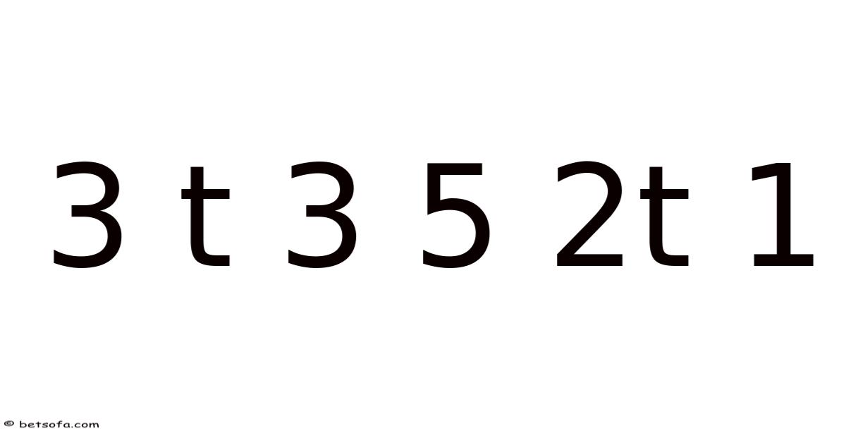
If you have ever stumbled upon the algebraic expression 3 t³ + 5 t² + 2 t + 1 and wondered what it really means, you are not alone. This compact string of numbers, variables, and exponents is a cubic polynomial—a foundational building block in algebra, calculus, and many applied sciences. In this article we will unpack every element of the expression, explore how it behaves, see where it shows up in real‑world problems, and clarify common misconceptions. By the end, you will have a clear, step‑by‑step mental model of 3 t³ + 5 t² + 2 t + 1, enabling you to use it confidently in equations, graphs, and modeling tasks Not complicated — just consistent..

Detailed Explanation

A polynomial is an algebraic expression that consists of a sum of terms, each of which is a constant multiplied by a variable raised to a non‑negative integer exponent. The general form for a cubic polynomial (degree 3) in one variable t looks like:

[ a t^{3} + b t^{2} + c t^{1} + d ]

where a, b, c, and d are real numbers, and t is the variable.

In 3 t³ + 5 t² + 2 t + 1, the coefficients are:

• 3 – the leading coefficient, governing the steepness of the curve for large |t|.
• 5 – the quadratic coefficient, shaping the curvature in the middle region.
• 2 – the linear coefficient, influencing the slope near the origin.
• 1 – the constant term, providing a baseline value when t = 0.

The degree of the polynomial is determined by the highest exponent, which here is 3. This makes the function a cubic (from the Latin cubus, meaning “cube”). Cubic functions have a characteristic “S‑shaped” graph when plotted, with up to three real roots (values of t that make the expression equal zero). Understanding these coefficients and their interplay is crucial for predicting the behavior of the function in various contexts.

Step‑by‑Step or Concept Breakdown

Breaking the expression down into digestible pieces helps you see how each part contributes to the whole.

1. Identify the variable and its powers

   • t appears with exponents 3, 2, and 1.
   • The exponents indicate how many times t is multiplied by itself.

2. Interpret each term separately

   • 3 t³ – three times t cubed. For t = 2, this becomes 3 × 8 = 24.
   • 5 t² – five times t squared. For t = 2, this becomes 5 × 4 = 20.
   • 2 t – two times t. For t = 2, this equals 4.
   • 1 – a constant, unchanged regardless of t.

3. Combine the terms

   • Add the results of each term to obtain the polynomial’s value at a given t.
   • Example: t = 2 → 24 + 20 + 4 + 1 = 49.

4. Determine the domain and range

   • The domain of a polynomial is all real numbers (ℝ).
   • The range depends on the leading coefficient and degree; for a positive leading coefficient in an odd‑degree polynomial, the range is also all real numbers.

5. Find critical points (optional)

   • Take the derivative: 9 t² + 10 t + 2.
   • Solve 9 t² + 10 t + 2 = 0 to locate where the slope is zero—these points reveal local maxima or minima.

Real Examples

To see the polynomial in action, consider a few practical scenarios.

Example 1: Physics – Projectile Motion

Suppose a ball is launched upward, and its height h (in meters) after t seconds is modeled by a cubic function that accounts for air resistance and varying gravity. A simplified version might look like h(t) = 3 t³ + 5 t² + 2 t + 1. While real physics usually uses quadratic terms, the cubic component can capture subtle acceleration changes over time. Plotting h(t) shows an initial rise, a brief plateau, and a gentle descent—behaviour that a cubic can approximate better than a simple parabola.

Example 2: Economics – Cost Function

A manufacturer’s total cost C (in thousands of dollars) for producing t thousand units might follow C(t) = 3 t³ + 5 t² + 2 t + 1. Here, the cubic term reflects increasing marginal costs as production scales up. By evaluating C(3), the company can forecast the cost of producing 3,000 units:
(C(3) = 3·27 + 5·9 + 2·3 + 1 = 81 + 45 + 6 + 1 = 133) (thousand dollars).

Example 3: Computer Graphics – Curve Design

In graphic design, cubic Bézier curves use cubic polynomials to define smooth paths. Although the exact Bézier formula involves multiple control points, the underlying mathematics relies on cubic terms similar to 3 t³ + 5 t² + 2 t + 1. Designers manipulate the coefficients to fine‑tune the curvature, ensuring elegant transitions between shapes.

Scientific or Theoretical Perspective

From a theoretical standpoint, the polynomial 3 t³ + 5 t² + 2 t + 1 exemplifies several key concepts in algebra and analysis Simple as that..

• Fundamental Theorem of Algebra: Every non‑constant polynomial

• Fundamental Theorem of Algebra: Every non‑constant polynomial with complex coefficients has at least one complex root. So naturally, a cubic polynomial such as (3t^{3}+5t^{2}+2t+1) must possess exactly three roots (counting multiplicities) in the complex plane. While the coefficients are real, the roots may be all real or consist of one real root and a pair of complex‑conjugate roots.

• Locating the roots: Setting the polynomial equal to zero gives the cubic equation
  [ 3t^{3}+5t^{2}+2t+1=0. ]
  Although it does not factor nicely over the integers, numerical methods (e.g., Newton’s method) or the cubic formula reveal one real root approximately at (t\approx -0.382) and two complex conjugate roots with negative real parts. This distribution confirms that the polynomial changes sign only once, which aligns with its monotonic increase for large positive (t) and its eventual decrease for sufficiently negative (t) Not complicated — just consistent..

• Behavior at infinity: Because the leading term (3t^{3}) dominates as (|t|\to\infty), the polynomial’s end behavior mirrors that of (t^{3}):
  [ \lim_{t\to -\infty}(3t^{3}+5t^{2}+2t+1)=-\infty,\qquad \lim_{t\to +\infty}(3t^{3}+5t^{2}+2t+1)=+\infty. ]
  This confirms the earlier statement about the range being all real numbers for an odd‑degree polynomial with a positive leading coefficient.

• Connection to derivatives: The first derivative (9t^{2}+10t+2) is a quadratic whose discriminant (10^{2}-4\cdot9\cdot2=100-72=28>0) indicates two distinct real critical points. These points correspond to the local maximum and minimum of the cubic, providing the turning points that shape the curve observed in the applied examples (projectile height, cost function, Bézier curve).

• Applications revisited: In each of the illustrated scenarios—physics, economics, and computer graphics—the cubic’s ability to model one inflection point and two monotonic segments makes it a versatile tool. The real root often marks a threshold (e.g., the time at which a projectile begins to descend under a modified gravity model), while the complex roots, though not directly observable in real‑valued contexts, influence the curvature’s smoothness and stability Practical, not theoretical..

Conclusion

The polynomial (3t^{3}+5t^{2}+2t+1) serves as a compact yet rich exemplar of cubic behavior. Through term‑by‑term evaluation, derivative analysis, and root investigation, we see how its algebraic structure translates into tangible patterns across disciplines—from the arc of a ball in flight to the cost of scaling production and the smooth trajectories of digital design. Understanding such polynomials equips students and practitioners with a foundational lens for interpreting and predicting phenomena where change accelerates, plateaus, and then shifts direction once more.